ggrebalance: Part 2. Planning a rebalance operation

Contents

2.1 User scenarios
2.2 Achieving uniform distribution. Formal cluster model
2.3 Analysis of methods for finding a balanced state
2.4 Comparison of selected approaches
2.5 Implementation in the ggrebalance utility
2.6 Resource assessment. Ports. Data volume
Conclusions

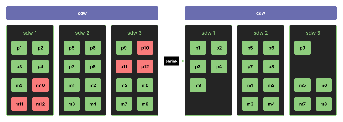
The previous article described in detail the procedure for removing a subset of segments from a Greengage cluster. After data redistribution and termination of unnecessary instances, the remaining segments may become unevenly distributed across hosts (Figure 1).

Figure 1. Cluster state after cutting off some segments

Uneven segment distribution across hosts, all else being equal, can degrade query performance. For example, if host sdw1 contains 4 primary segments while sdw3 contains only 1, queries processing large volumes of data will consistently run slower on sdw1 because of its proportionally higher I/O and CPU load, as well as increased memory consumption. This is a common issue in MPP storage systems. Mirror distribution can make this problem worse in a similar way. Regardless of the mirroring strategy initially chosen, skew in primary segment distribution after cluster shrink leads to corresponding skew in mirror segment distribution. If one of the hosts fails, the promotion of replicas can further degrade overall system performance. In turn, uniform segment distribution makes cluster resource planning more convenient and predictable. Thanks to the uniform cluster structure, each host requires the same amount of memory, the same port range, and the same disk capacity. This simplifies integration with monitoring and automation systems.

In addition to segment shrinking, there are several scenarios directly related to managing cluster hosts. Engineers may need to decommission individual hosts for maintenance, replacement, cost optimization, or resource reallocation, as well as add new hosts to scale the workload (Figures 2 and 3). In such cases, Greengage does not automatically redistribute segments: neither from a host being removed nor to a host being added.

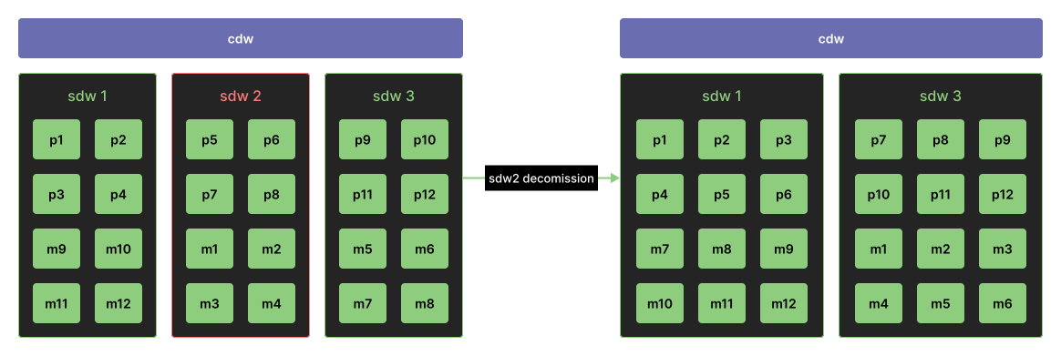
Figure 2. Decommissioning a host

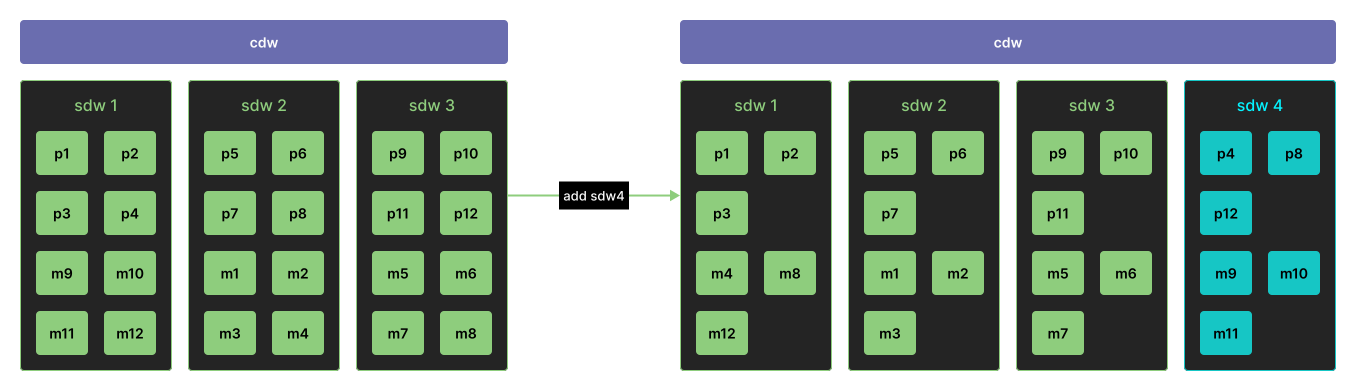
Figure 3. Adding a host

In all described scenarios, the end goal is the same: to achieve a segment distribution where each active or newly added host contains the same number of primary segments and replicas while preserving the selected mirroring topology (Grouped or Spread).

Assume the cluster has m hosts, n primary segments, and n mirror segments. Denote the set of hosts by , and the sets of segments and mirrors by and , respectively. For simplicity, introduce the corresponding index sets: — indices of both segments and mirrors, and — a set of host indices.

In Greengage terminology, there are two mirroring strategies: Grouped and Spread. The Grouped strategy means that for a set of segments running on one host, all corresponding mirrors are located on a single host (different from the primary host). A set of segments located on the same host is called a primary group. The Spread strategy, in turn, means that for any primary group of size k, the corresponding mirrors are distributed across k different hosts.

Let us introduce the notation used to describe a cluster configuration. The following set of mappings is called the cluster configuration:

These mappings uniquely determine the placement of each primary and mirror segment across the cluster hosts. Therefore, the initial state of the cluster shown in Figure 1 can be represented as follows:

By the fill (or load) of host h, we mean the following value:

A cluster configuration is considered balanced if it is in a state such that .

The primary group of host is the set . Using this definition, we can introduce the concept of a feasible cluster configuration. A state is feasible if the following conditions are satisfied:

Let q denote the target number of segments per host. The set of possible states is defined as .

Cluster balancing is the process of transforming an arbitrary initial state into a balanced final state. Since moving a single segment is a time-consuming operation (the movement process is described in more detail in the third part of this article and often involves a backup/restore sequence), balancing a cluster with production-scale data volumes may require significant time. Therefore, the goal is to minimize the number of segment transfers required to bring the system to a balanced state. Given these premises, the rebalance operation can be formulated as the following optimization problem: transform the initial cluster state into a balanced state while minimizing the number of moves. Formally:

— initial state

Find such that:

This problem belongs to the field of combinatorial optimization and can be reduced to a mixed-integer linear programming (MILP) problem. The corresponding decision problem is NP-complete. This classification matters in practice because of the computational complexity of solving the problem: the computation time grows exponentially with increasing problem size. In this context, small clusters can be considered to contain up to 60 segments, medium-sized clusters from 60 to 300 segments, and large industrial analytical systems with more than 300 segments (typically not exceeding 1000). Even with these seemingly reasonable constraints, the space of possible solutions remains enormous. This makes relying solely on exact algorithms impractical. Therefore, approximate heuristic and metaheuristic methods are often used.

To address the rebalance problem, whose goal is to achieve an even distribution of segments across hosts while minimizing segment movements, we analyzed the following exact and metaheuristic methods.

MILP-based exact solver (PuLP + CBC)

The first approach is to use an existing exact solver for the MILP formulation of the problem. The PuLP Python package was selected for this purpose. It solves MILP problems using the CBC solver, which combines branch-and-bound with cutting-plane methods. This is an exact algorithm with exponential complexity, although it incorporates some heuristics. The MILP formulation of our problem is based on straightforward linearization:

Exact methods are used in the analysis to obtain exact values of the minimum number of moves and demonstrate the quality loss of faster heuristic methods. During linearization, the model accumulates different constraints, causing the algorithm to perform poorly already at medium values of n.

Exact CP-SAT solver (Google OR-Tools)

The second exact approach uses the CP-SAT solver from the Google OR-Tools toolkit and is based on the Constraint Programming paradigm. CP-SAT is better suited for problems with a large number of constraints, which can also be expressed more naturally in this framework.

Greedy algorithm (GreedyRebalance)

The greedy algorithm implements an intuitive balancing approach: it places segments in a way similar to how a user might do so manually.

The algorithm consists of two steps. Line 1 of the pseudocode calls BalancePrimaries, which redistributes primary segments across hosts so that each host contains exactly n/m primary segments. This step uses a greedy strategy: it iterates over hosts with excess segments and moves segments to hosts with a deficit until the load is balanced. No exhaustive search is performed; the algorithm requires only a single linear pass while accounting for host decommissioning or addition.

After primary segments are balanced, AssignMirrors is called to place mirror segments based on the fixed placement of primary segments and the initial mirror placement . The algorithm attempts to keep each mirror on its original host whenever this does not violate the mirroring strategy, thereby minimizing the number of mirror movements. The result is a configuration that is guaranteed to satisfy all constraints described in section 2.2. The overall algorithm complexity is with .

Multiple runs of the greedy algorithm with random initialization

This variant repeatedly runs the greedy algorithm from randomly generated initial configurations. After k iterations, the best resulting configuration is selected. Although this approach may provide a small improvement due to randomness, it does not perform a systematic search of the solution space.

Simulated annealing algorithm

The Simulated Annealing method is a metaheuristic approach for solving optimization problems. The simulated annealing algorithm is inspired by the behavior of atoms in metals during the annealing process (Algorithm 2).

The naive (greedy) solution serves as a warm start for the algorithm, providing a reasonable initial solution and significantly reducing the time required to reach a promising region of the search space.

(a hyperparameter) is the initial temperature that determines the probability of accepting deteriorating moves at the beginning of the search, allowing the algorithm to escape local extrema. On each iteration, the Move method randomly moves a primary or mirror segment, optionally validates the feasibility conditions, and returns a new cluster configuration.

is the objective function that represents the number of segments whose host in configuration differs from the corresponding host in the original configuration . Line 8 specifies the key acceptance rule: an improving move is always accepted, while a worsening move is accepted with probability . The greater the deterioration and the lower the temperature , the lower the acceptance probability.

The divisor n normalizes the objective difference by the problem size, ensuring that the parameters and remain independent of the number of segments.

defines geometric cooling with coefficient . At each iteration, the temperature decreases, making the algorithm increasingly greedy and reducing the probability of accepting worsening moves. The algorithm continues searching for improvements until the final iteration .

Tabu search

Tabu Search is a metaheuristic optimization method based on local search. In our implementation, it partially incorporates ideas from the simulated annealing algorithm.

In line 1, as in simulated annealing, the algorithm uses a warm start based on a greedy solution. In line 2, the tabu list is initialized as a dictionary of the form {configuration key → iteration number until which the configuration is forbidden}. An entry means that the corresponding cluster state variant cannot be used until iteration .

At each iteration of the main loop, line 4 calls GenerateCandidates( ) (Algorithm 4), which generates a set of candidate neighbors of configuration . In line 5, the best candidate according to the objective function is selected, provided it satisfies at least one of two conditions: the move is not forbidden, or the move yields the best solution. This prevents the algorithm from missing the best solution due to the prohibition logic. If there are no admissible candidates, the iteration is skipped (line 6). In line 8, the selected move is added to the tabu list for the next iterations. This prevents an immediate return to the previous configuration and encourages the algorithm to explore new regions of the search space. Lines 9—12 update the current solution and the best solution found so far.

GenerateCandidates builds the neighborhood as follows: the first half of the candidate set ( candidates, lines 3—11) consists of primary segment moves. A segment s is chosen at random and moved to a target host selected from the set of hosts . For the Grouped strategy, the entire primary group is moved together as a single unit.

The second half of the candidate set (lines 13—24) consists of mirror segment moves, whose logic depends on the mirroring strategy. For the Grouped strategy, a target host is selected to which the entire mirror group can be moved without violating the primary/mirror co-location constraint. For the Spread strategy, the target host must differ from both the segment’s primary host and the hosts containing other mirrors of the same content. The set of already visited keys prevents duplicate moves within a single iteration. Each candidate is checked for feasibility , and invalid configurations are discarded immediately.

Large neighborhood search (LNS)

As a baseline LNS method (Large Neighborhood Search), we implement the PlainLNS algorithm (Algorithm 5) with a warm start from a greedy solution. At each iteration, the destruction operator removes a random fraction of segments from the current solution. The repair operator then constructs a complete feasible configuration by filling the freed positions. Both operators are selected uniformly at random from a fixed set (Table 1). The acceptance criterion is greedy: improving solutions are always accepted, while solutions with equal objective values are accepted with probability .

Table 1. Destruction and repair operators
Type	Operator	Applicable strategy
Destroy	Group destruction	Grouped
	Bad segments	Both
	Shaw removal	Both
	Random segments	Both
Repair	Greedy repair	Both
	Most constrained repair	Both
	Regret-based repair	Both

Destroy operators work as follows:

The "Random segments" removal operator removes uniformly selected segments, producing configuration .
"Bad segments" targets segments whose current placement deviates the most from the initial configuration. The distance is discrete: 0 — neither the primary nor the mirror has been moved from the original configuration; 1 — one of the two placements (primary or mirror) differs from the original; 2 — both the primary and mirror placements differ from the original.
"Shaw removal" removes a group of mutually similar segments (segments sharing a primary or mirror host).
"Group destruction" (only available for the Grouped strategy) removes all segments belonging to a randomly selected subset of primary groups.

All repair operators reassign primary and mirror hosts for each segment in , restoring the feasibility constraints (1)-(3) from section 2.2:

"Greedy repair" assigns hosts in descending order of a load deficit.
"Most constrained repair" processes segments with the fewest valid placement options first.
"Regret-based repair" prioritizes segments for which the cost difference between the best and second-best host assignments is the largest.

Adaptive large neighborhood search (ALNS)

ALNS (Adaptive Large Neighborhood Search) extends the LNS approach through adaptive operator selection (Algorithm 6). The algorithm starts from the solution produced by the greedy method and iteratively improves it by alternating between destroy and repair operators. A key feature of the method is adaptive operator selection: each operator is assigned a weight that is updated every iterations based on its accumulated score using exponential smoothing with reaction factor . Operators that consistently produce improvements receive higher weights and are selected with higher probability.

The acceptance criterion is based on the simulated annealing method: a worsening move with cost difference is accepted with probability , where the temperature decreases logarithmically from to . The destruction size adapts to the search phase: large neighborhoods are used at the beginning of the search to explore the solution space, while smaller neighborhoods are used later for intensification. In case of stagnation, the current solution is reset to the best solution found so far. After the main loop completes, a final local search is applied to the best solution, but only for the Grouped strategy: mirror hosts are swapped between groups.

In total, eight algorithms are considered: two exact solvers (MILP with PuLP+CBC and CP-SAT), used at small scales to evaluate the improvement achieved by the others; a greedy algorithm; greedy with random restarts; simulated annealing; tabu search; standard LNS without adaptation; ALNS. All algorithms are run on the same sample of configuration instances of different sizes with the same seed values.

Tasks are classified by three cluster sizes — small, medium, and large — and by two mirroring strategies: Grouped and Spread. Additionally, three operational scenarios are considered: balancing without changing the number of hosts, decommissioning hosts, and adding new hosts. For small clusters, where exact methods can find the optimum within the time limit, the optimality gap is used as the quality metric: the percentage by which a solution is worse than the exact optimum. For medium and large clusters, where exact methods are too slow and exceed the configured timeout (300 s), the improvement factor relative to the greedy solution is used: the percentage reduction in the number of movements compared with the greedy baseline. The time required to reach the best solution found is also recorded.

The table below describes the datasets used in the comparative experiments.

Table 2. Number of configurations in experiments. Total of 170 different initial states
Set	Number of configurations	Number of seeds	Total configurations	Number of primary
small_grouped	4	5	20	12—48
small_spread	4	5	20	12—48
medium_grouped	4	5	20	100—320
medium_spread	4	5	20	80—240
large_grouped	4	5	20	256—1024
large_spread	4	5	20	224—930
decommission_grouped	3	5	15	120—500
decommission_spread	2	5	10	120—200
expansion_grouped	3	5	15	120—540
expansion_spread	2	5	10	120—200

Consider the comparison results for small-scale instances. Exact methods are included as optimality baselines. The small_grouped and small_spread sets were used for collecting statistics, comprising 40 instances and 360 runs in total. The improvement rate is calculated as:

Here, denotes the number of moves performed by the evaluated algorithm, while denotes the number of moves in the optimal solution obtained by the exact algorithm (CBC or CP-SAT).

Table 3. Gap to optimum, % (compared to exact methods) on small instances
Algorithm	IR, %	IRmax, %
ALNS	0.00	0.00
PlainLNS	0.00	0.00
SA	0.00	0.00
RandomRestart	5.43	38.10
Tabu	7.00	50.00
Greedy	10.00	50.00

The table shows that three algorithms — ALNS, PlainLNS, and SA — achieve a zero optimality gap for all small configurations. In other words, they find the optimal solution in every case. The greedy algorithm is, on average, 10% worse than the optimum, while RandomRestart and Tabu are 5.4% and 7% worse, respectively. For small problem instances, even simple LNS and SA are sufficient to achieve optimality; no complex adaptive mechanism is required.

Next, consider experiments with medium and large values of n. Due to the significant slowdown of exact algorithms caused by the exponential growth of the search space, the comparison is based on improvements relative to the greedy approach. The evaluated sets are medium_grouped, medium_spread, large_grouped, and large_spread. In total, 80 instances and 560 runs are included in the evaluation.

Table 4. Gap to the cost of the naive algorithm. Medium and large configurations
Algorithm	Strategy	IR, %	Standard deviation
ALNS	spread	21.47	5.24
PlainLNS	spread	21.83	4.78
SA	spread	6.00	9.13
RandomRestart	spread	0.22	0.83
Tabu	spread	5.43	9.19
ALNS	grouped	0.25	1.26
PlainLNS	grouped	0.22	1.23
SA	grouped	0.49	1.54
RandomRestart	grouped	0.22	1.23
Tabu	grouped	0.80	1.68

This is the most significant result of the entire study: the Grouped and Spread strategies exhibit fundamentally different behavior. For the Grouped strategy, the greedy algorithm already produces a near-optimal solution: none of the methods improves the result by more than 0.8%, and the median improvement is zero for all methods. This can be explained by the structure of the problem: in the Grouped variant, mirror placement is determined by a single permutation mapping, and after the primary segment balancing phase, little room for further optimization remains. For the Spread strategy, the situation is fundamentally different. The greedy algorithm leaves a gap of approximately 22—23% relative to the optimum, while PlainLNS (21.83%) and ALNS (21.47%) recover almost the entire gap; both methods are statistically significantly better than the greedy baseline. SA achieves only a 6% improvement, while RandomRestart improves the result by less than 0.3%, which is effectively negligible.

Thus, the greedy algorithm provides the best results for the Grouped strategy on medium and large configurations. As an initial solution, its output is more than sufficient for planning segment movements with the ggrebalance utility. Nevertheless, reducing the number of movements by even a few operations can still be beneficial, especially for the Spread strategy, where substantial room for improvement remains. At this stage, PlainLNS and ALNS demonstrate the best results. The remaining question is whether LNS adaptivity is actually necessary for this task. The Wilcoxon signed-rank test can be used to answer this question. Among 40 paired observations from the medium_grouped and medium_spread sets, ALNS outperforms PlainLNS only once, PlainLNS outperforms ALNS three times, and the remaining 36 cases produce identical results. The Wilcoxon signed-rank test yields p = 0.705, indicating no statistically significant difference. This suggests that the adaptive operator selection mechanism, including weight updates and exponential smoothing, does not provide a practical advantage for this class of problems. A possible explanation is that the search space is sufficiently homogeneous and all operators have comparable effectiveness, leaving little useful information for the adaptation mechanism to learn.

Finally, Figure 4 shows how the solution search time of all methods depends on the problem size.

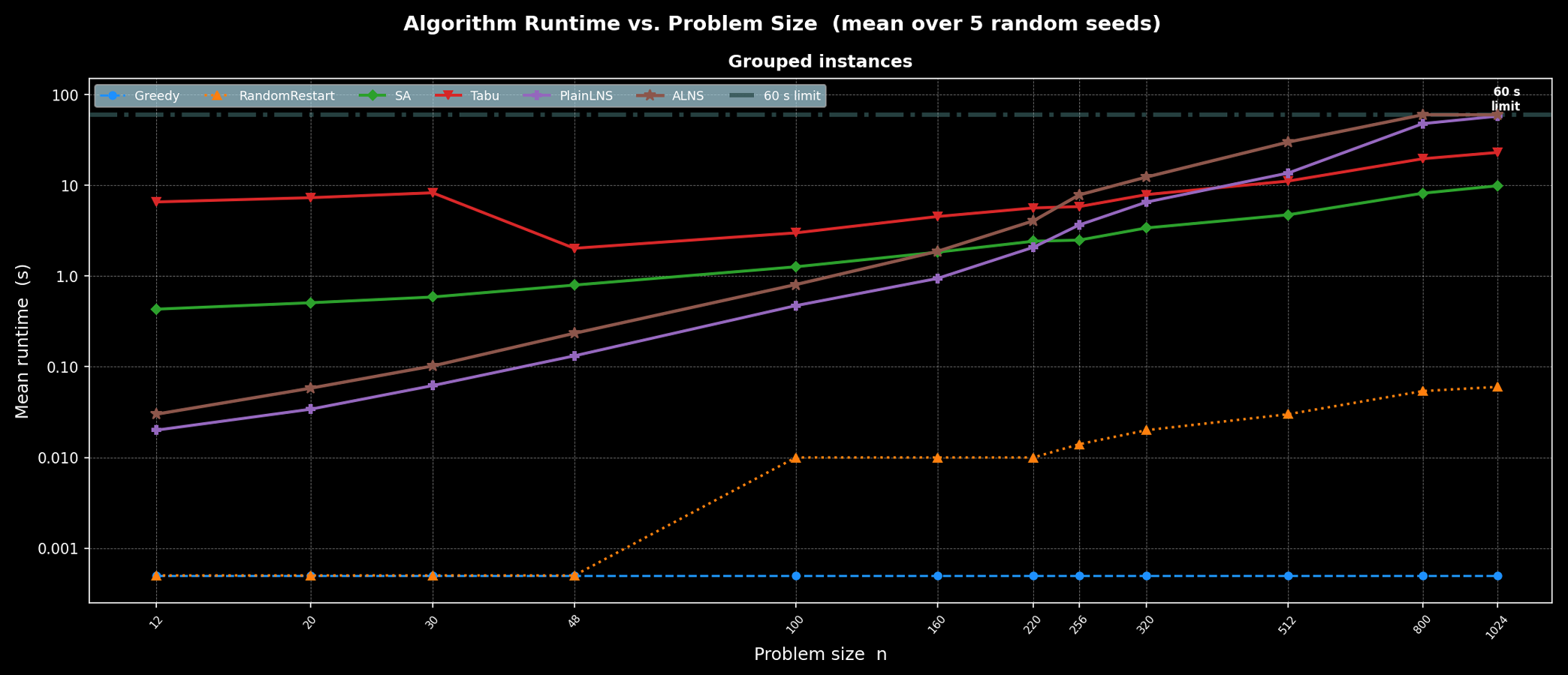
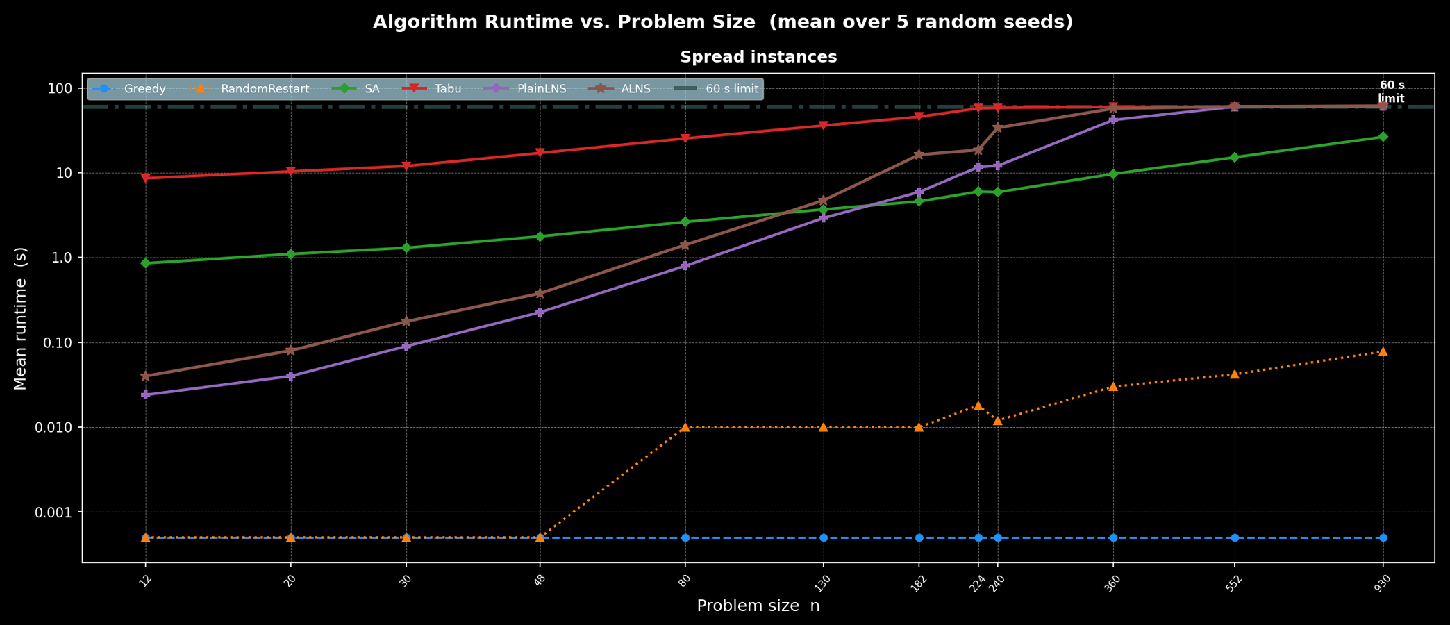
Figure 4. Execution time dependency on problem dimension

Based on the comparative analysis, the non-adaptive PlainLNS search method is selected as the primary candidate for the Greengage cluster balancing task.

The planning module (planner.py) implements the logic for generating a rebalance plan for Greengage cluster segments. A brief component diagram illustrating the operation planning process is shown in Figure 5. The central class is Planner, which accepts the current cluster state from gp_segment_configuration and a set of startup parameters, and builds a Plan object — a list of logical moves (LogicalMove) required to reach a balanced state. The plan is generated by the plan() method, which sequentially performs several stages. First, the status of all segments is checked. The presence of any segment in the down state immediately stops the planning process, because rebalancing a partially unavailable cluster is unsafe. Next, if required, a reduction in the number of segments (shrink) is planned. After that, unless the --skip-rebalance flag is specified, the actual segment movements are planned.

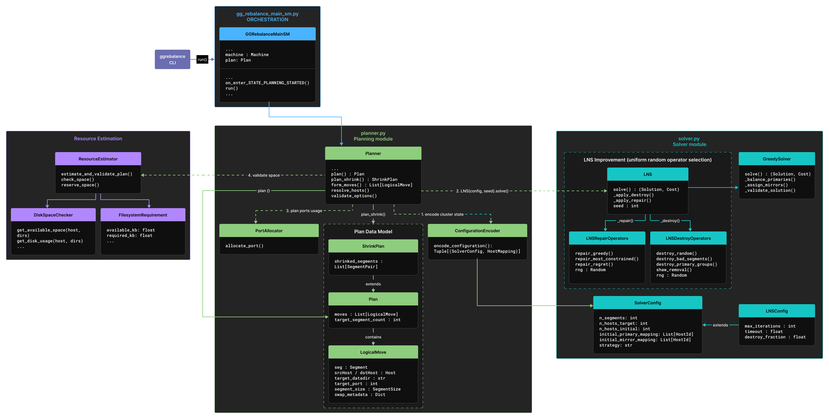
Figure 5. ggrebalance planner components

Before solving the balancing problem, the planner builds the complete set of hosts involved in the operation. Each host is represented by an object with one of the following statuses: active (an existing cluster host), new (a host being added), or decommissioned (a host being removed from the cluster).

Command-line parameters — --target-hosts, --add-hosts, and --remove-hosts — are translated into these statuses. If --target-hosts is specified, all existing hosts not included in the list are marked as decommissioned, while hosts from the list that are absent from the cluster are marked as new. The --add-hosts parameter adds new hosts with the new status, and --remove-hosts marks existing hosts as decommissioned.

For each host, data directory path templates are also stored and used to generate target paths for moved segments. The utility resolves host names and addresses, allowing hosts to be specified by either hostname or IP address.

Next, the cluster representation based on gp_segment_configuration is converted into an abstract numeric representation similar to and passed to the PlainLNS solver, which contains GreedyBalancer and improves its result using LNS. The final balanced configuration becomes the target state for plan generation. The solver output is compared with the initial placement. For each segment whose host assignment has changed, a LogicalMove object is created.

Each move requires assigning a port for the segment on the target host. A separate class handles this process: during initialization, it collects all occupied ports from gp_segment_configuration and separately tracks the ports used by primary and mirror segments. When allocating a port on an existing host, the planner first attempts to reuse the segment’s current port. If the port is available on the target host, it is assigned to the moved segment. This approach minimizes configuration changes. If the port is already in use, the planner searches for the next available port, starting from the base port assigned to the given role (primary or mirror) on the target host. For new hosts, the first segment of each role defines the base port, which is then used to assign ports to subsequent segments. This approach ensures a consistent port allocation scheme and prevents conflicts in the planned configuration. During port allocation, the target host is also queried to verify that the port is available. Therefore, each move requires a network request, increasing the planning overhead. This check can be skipped by passing the --skip-resource-estimation option.

However, port validation during planning does not strictly guarantee that the selected port will remain available at the operating system level when the relocation is executed: between the planning and execution stages, the port may be occupied by an external process or become unavailable due to environmental changes. Therefore, the rebalance operation should be performed within a controlled change window, and the required port range should be reserved for new hosts in advance. Otherwise, execution may fail; this does not cause serious consequences but requires restarting the utility and administrator intervention.

During planning, it is also important to determine the amount of data, including all tablespaces, that needs to be moved and verify that the target hosts have sufficient capacity for additional segments. This is true even when another segment on the same host is scheduled to move away, because its data remains in place until that relocation is completed. Therefore, the ggrebalance planner performs this initial check. The estimation is performed in two steps. In the first step, parallel SSH requests using du are sent to the source hosts to determine the sizes of the data directories of all segments being moved. Additionally, an SQL query is executed against the cluster to retrieve the tablespace locations used by the moved segments; their sizes are also collected. In the second step, information about available disk space on the target hosts is collected. All planned moves are aggregated by file system on the target hosts. This is important because multiple data directories can reside on the same file system, and the total required space must be compared with the free space available on that file system rather than with the capacity of individual directories.

The safety margin DISK_SPACE_SAFETY_MARGIN (10%) is applied to the estimated size, increasing the required capacity. This margin compensates for estimation errors and file system overhead. If any host does not have sufficient space, a detailed error message is generated with a breakdown by file systems, directories, and affected segments. After successful validation, the amount of data planned for movement is written to the log. Space usage estimation can also be skipped by using the --skip-resource-estimation option.

Thus, taking the configuration shown in Figure 1 (after shrink) as the initial state:

select hostname,role, array_agg(content) from gp_segment_configuration group by hostname, role order by hostname;
hostname | role |  array_agg
----------+------+-------------
cdw      | p    | {-1}
sdw1     | p    | {0,1,2}
sdw1     | m    | {8,3}
sdw2     | m    | {0,1,2}
sdw2     | p    | {5,6,4,7,3}
sdw3     | m    | {5,6,4,7}
sdw3     | p    | {8}
(7 rows)

ggrebalance produces the following plan:

20260412:20:09:41:014374 ggrebalance:cdw:gpadmin-[INFO]:-Final plan:

------------------------BALANCE MOVES--------------------------------
Total moves planned: 4

  [1] Move Segment(content=3, dbid=5, role=p) [834.81 MB]
      From: sdw1:7005:/home/gpadmin/.data/primary/gpseg3
      To:   sdw3:7005:/home/gpadmin/.data/primary/gpseg3

  [2] Move Segment(content=3, dbid=14, role=m) [834.26 MB]
      From: sdw2:7053:/home/gpadmin/.data/mirror/gpseg3
      To:   sdw1:7053:/home/gpadmin/.data/mirror/gpseg3

  [3] Move Segment(content=7, dbid=9, role=p) [834.26 MB]
      From: sdw2:7009:/home/gpadmin/.data/primary/gpseg7
      To:   sdw3:7009:/home/gpadmin/.data/primary/gpseg7

  [4] Move Segment(content=7, dbid=18, role=m) [833.71 MB]
      From: sdw3:7057:/home/gpadmin/.data/mirror/gpseg7
      To:   sdw1:7057:/home/gpadmin/.data/mirror/gpseg7

It describes the steps required to bring the cluster into a balanced state, including target directories for data placement and an estimate of the data volume to be moved.

This work addressed the problem of rebalancing Greengage cluster segments after shrink operations, as well as in host decommissioning and addition scenarios. Unlike simple segment decommissioning, this operation requires not only physical data movement but also the construction of a valid target configuration that preserves the placement of primary and mirror segments, complies with the selected mirroring strategy, and achieves an even load distribution across all active hosts.

To formalize the problem, a cluster configuration model was introduced using mappings that define the placement of primary and mirror segments across the set of hosts. Based on this model, the rebalance problem was formulated as a combinatorial optimization problem with an objective function that minimizes the number of segment movements. The analysis of exact methods showed that they are suitable as benchmarks for small-scale problems but become computationally impractical as the number of segments increases. This justifies the transition to heuristic and metaheuristic approaches.

The practical value of ggrebalance is that it fills an important gap in Greengage cluster management: after cluster scaling operations (such as shrink), it brings the system to a predictable and operationally convenient state. An even distribution of primary and mirror segments reduces the risk of performance degradation, simplifies resource planning, makes the cluster configuration more uniform, and facilitates maintenance by administrators, monitoring systems, and automation tools.

The third and final article in this series will examine the process of moving segment data between hosts in detail and demonstrate cluster topology change scenarios involving host decommissioning and addition.

Blog

Major Greengage upgrade using pg_upgrade and ggupgrade

ggrebalance: Part 2. Planning a rebalance operation

2.1 User scenarios

2.2 Achieving uniform distribution. Formal cluster model

2.3 Analysis of methods for finding a balanced state

2.4 Comparison of selected approaches

2.5 Implementation in the ggrebalance utility

2.6 Resource assessment. Ports. Data volume

Conclusions